One way to make your data a little easier to read is with the help of alternating row colors. This additional formatting choice will make all of the cells in the same row a certain color, which can make those cells much easier to identify when they are far away from the header. Our tutorial below will show you how to apply this formatting automatically to the data in a Google Sheets spreadsheet.
How to Automatically Make Rows Alternating Colors in Google Sheets
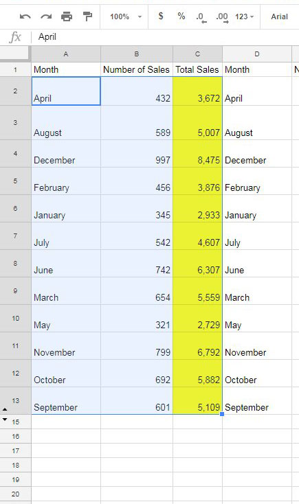
The steps in this guide were performed in the desktop version of Google Chrome,. but will also work in other desktop browsers like Firefox and Edge. By completing the steps in this guide you will select some cells in your spreadsheet and apply a pattern of fill colors to that selection, where each row will be a different, alternating color. You will have the option to customize these colors if you wish. Step 1: Sign into your Google Drive and open the Sheets file to which you want to apply alternating colors. Step 2: Select the cells to which you wish to apply this formatting.
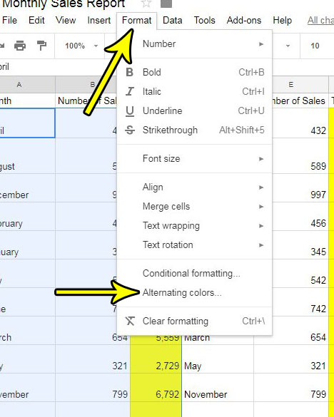
Step 3: Click the Format tab at the top of the window, then choose the Alternating Colors option at the bottom of the menu.
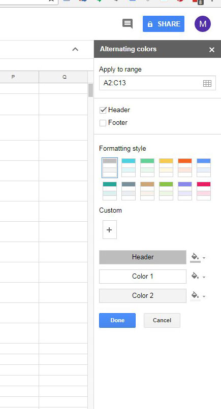
Step 4: Choose one of the default color schemes in the column at the right side of the window, or set your own custom colors in the section at the bottom of the menu. You can also check or uncheck the Header or Footer options if you would like to make those rows a different color than the data that you are formatting. Once you’re finished click the Done button at the bottom of the column.
Do you need to make some of your cells bigger but you don’t want to affect other cells in nearby columns or rows? Find out how to merge cells in Google Sheets to make larger cells within your spreadsheet. He specializes in writing content about iPhones, Android devices, Microsoft Office, and many other popular applications and devices. Read his full bio here.


